(Thanks to Bill Rosgen and Edwin Chen for help preparing these notes.)
We're going to start by beating a retreat from QuantumLand, back onto the safe territory of computational complexity. In particular, we're going to see how in the 80's and 90's, computational complexity theory reinvented the millennia-old concept of mathematical proof -- making it probabilistic, interactive, and cryptographic. But then, having fashioned our new pruning-hooks (proving-hooks?), we're going to return to QuantumLand and reap the harvest. In particular, I'll show you why, if you could see the entire trajectory of a hidden variable, then you could efficiently solve any problem that admits a "statistical zero-knowledge proof protocol," including problems like Graph Isomorphism for which no efficient quantum algorithm is yet known.
What Is A Proof?
Historically, mathematicians have had two very different notions of "proof."
The first is a that a proof is something that induces in the audience (or at least the prover!) an intuitive sense of certainty that the result is correct. On this view, a proof is an inner transformative experience -- a way for your soul to make contact with the eternal verities of Platonic heaven.
The second notion is that a proof is just a sequence of symbols obeying certain rules -- or more generally, if we're going to take this view to what I see as its logical conclusion, a proof is a computation. In other words, a proof is a physical, mechanical process, such that if the process terminates with a particular outcome, then you should accept that a given theorem is true. Naturally, you can never be more certain of the theorem than you are of the laws governing the machine. But as great logicians from Leibniz to Frege to Gödel understood, the weakness of this notion of proof is also its strength. If proof is purely mechanical, then in principle you can discover new mathematical truths by just turning a crank, without any understanding or insight. (As Leibniz imagined legal disputes one day being settled: "Gentlemen, let us calculate!")
The tension between the two notions of proof was thrown into sharper relief in 1976, when Kenneth Appel and Wolfgang Haken announced a proof of the famous Four-Color Map Theorem (that every planar map can be colored with four colors, in such a way that no two adjacent countries are colored the same). The proof basically consisted of a brute-force enumeration of thousands of cases by computer; there's no feasible way for a human to apprehend it in its entirety.
Answer: Good question! The novel technical contribution that human mathematicians had to make was precisely that of reducing the problem to finitely many cases -- specifically, about 2000 of them -- which could then be checked by computer. Increasing our confidence is that the proof has since been redone by another group, which reduced the number of cases from about 2000 to about 1000.
Now, people will ask: how do you know that the computer didn't make a mistake? The obvious response is that human mathematicians also make mistakes. I mean, Roger Penrose likes to talk about making direct contact with Platonic reality, but it's a bit embarrassing when you think you've made such contact and it turns out the next morning that you were wrong!
We know the computer didn't make a mistake because we trust the laws of physics that the computer relies on, and that it wasn't hit by a cosmic ray during the computation. But in the last 20 years, there's been the question -- why should we trust physics? We trust it in life-and-death situations every day, but should we really trust it with something as important as proving the Four-Color Theorem? The truth is, we can play games with the definition of proof in order to expand it to unsettling levels, and we'll be doing this for the rest of the lecture.
Probabilistic Proofs
Recall that we can think of a proof as a computation -- a purely mechanical process that spits out theorems. But what about a computation that errs with 2-1000 probability -- is that a proof? That is, are BPP computations legitimate proofs? Well, if we can make the probability of error so small that it's more likely for a comet to suddenly smash our computer into pieces than for our proof to be wrong, it certainly seems plausible!
Now do you remember our definition of NP, as the class of problems with polynomial-size certificates (for positive answers) that can be verified in polynomial time? In other words, it's the class of problems we can efficiently prove and check. So once we admit probabilistic algorithms as proofs, we should combine them with NP to get MA (named by Laszlo Babai after Merlin and Arthur), the class of problems with proofs efficiently verifiable by some randomized algorithm.
We can also consider the class where you get to Ask Merlin a question -- this is AM. What happens if you get to ask Merlin more than one question? You'd think you'd be able to solve more problems or prove more theorems, right? Wrong! It turns out that if you get to ask Merlin a constant number of questions, say, AMAMAM, then you have exactly the same power as just asking him once.
Zero-Knowledge Proofs
I was talking before about stochastic proofs, proofs that have an element of uncertainty about them. We can also generalize the notion of proof to include zero-knowledge proofs, proofs where the person seeing the proof doesn't learn anything about the statement in question except that it's true.
Intuitively that sounds impossible, but I'll illustrate this with an example. Suppose we have two graphs. If they're isomorphic, that's easy to prove. But suppose they're not isomorphic. How could you prove that to someone, assuming you're an omniscient wizard?
Simple: Have the person you're trying to convince pick one of the two graphs at random, randomly permute it, and send you the result. That person then asks: "which graph did I start with?" If the graphs are not isomorphic, then you should be able to answer this question with certainty. Otherwise you'll only be able to answer it with probability 1/2. And thus you'll almost surely make a mistake if the test is repeated a small number of times.
This is an example of an interactive proof system. Are we making any assumptions? We're assuming you don't know which graph the verifier started with, or that you can't access the state of his brain to figure it out. Or as theoretical computer scientists would say, we're assuming you can't access the verifier's "private random bits."
What's perhaps even more interesting about this proof system is that the verifier becomes convinced that the graphs are not isomorphic without learning anything else! In particular, the verifier becomes convinced of something, but is not thereby enabled to convince anyone else of the same statement.
A proof with this property -- that the verifier doesn't learn anything besides the truth of the statement being proved -- is called is called a zero-knowledge proof. Yeah, alright, you have to do some more work to define what it means for the verifier to "not learn anything." Basically, what it means is that, if the verifier were already convinced of the statement, he could've just simulated the entire protocol on his own, without any help from the prover.
Under a certain computational assumption -- namely that one-way functions exist -- it can be shown that zero-knowledge proofs exist for every NP-complete problem. This was the remarkable discovery of Goldreich, Micali, and Wigderson in 1986.
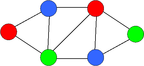
Because all NP-complete problems are reducible to each other (i.e., are "the same problem in different guises"), it's enough to give a zero-knowledge protocol for one NP-complete problem. And it turns out that a convenient choice is the problem of 3-coloring a graph (meaning: coloring every vertex red, blue, or green, so that no two neighboring vertices are colored the same).
The question is: how can you convince someone that a graph is 3-colorable, without revealing anything about the coloring?
Well, here's how. Given a 3-coloring, first randomly permute the colors -- for example by changing every blue country to green, every green country to red, and every red country to blue. (There are 3!=6 possible permutations.) Next, use a one-way function (whose existence we've assumed) to encrypt the color of every country. Then send the encrypted colors to the verifier.
Given these encrypted colors, what can the verifier do? Simple: he can pick two neighboring vertices, ask you to decrypt the colors, and then check that (1) the decryptions are valid and (2) the colors are actually different. Note that, if the graph wasn't 3-colorable, then either two adjacent countries must gotten the same color, or else some country must not even have been colored red, blue, or green. In either case, the verifier will catch you cheating with probability at least 1/m, where m is the number of edges.
Finally, if the verifier wants to increase his confidence, we can simply repeat the protocol a large (but still polynomial) number of times. Note that each time you choose a fresh permutation of the colors as well as fresh encryptions. If after (say) m3 repetitions, the verifier still hasn't caught you cheating, he can be sure that the probability you were cheating is vanishingly small.
But why is this protocol zero-knowledge? Intuitively it's "obvious": when you decrypt two colors, all the verifier learns is that two neighboring vertices were colored differently -- but then, they would be colored differently if it's a valid 3-coloring, wouldn't they? Alright, to make this more formal, you need to prove that the verifier "doesn't learn anything," by which we mean that by himself, in polynomial time, the verifier could've produced a probability distribution over sequences of messages that was indistinguishable, by any polynomial-time algorithm, from the actual sequence of messages that the verifier exchanged with you. As you can imagine, it gets a bit technical.
Is there any difference between the two zero-knowledge examples I just showed you? Sure: the zero-knowledge proof for 3-coloring a map depended crucially on the assumption that the verifier can't, in polynomial time, decrypt the map by himself. (If he could, he would be able to learn the 3-coloring!) This is called a computational zero-knowledge proof, and the class of all problems admitting such a proof is called CZK. By contrast, in the proof for Graph Non-Isomorphism, the verifier couldn't cheat even with unlimited computational power. This is called is a statistical zero-knowledge proof, a proof in which the distributions given by an honest prover and a cheating prover need to be close in the statistical sense. The class of all problems admitting this kind of proof is called SZK.
Clearly SZK⊆CZK, but is the containment strict? Intuitively, we'd guess that CZK is a larger class, since we only require a protocol to be zero-knowledge against polynomial-time verifiers, not verifiers with unlimited computation. And indeed, it's known that if one-way functions exist, then CZK = IP = PSPACE -- in other words, CZK is "as big as it could possibly be." On the other hand, it's also known that SZK is contained in the polynomial hierarchy. (In fact, under a derandomization assumpition, SZK is even in NP∩coNP).
PCP
A PCP (Probabilistically Checkable Proof) is yet another impossible-seeming game one can play with the concept of "proof." It's a proof that's written down in such a way that you, the lazy grader, only need to flip it open to a few random places to check (in a statistical sense) that it's correct. Indeed, if you want very high confidence (say, to one part in a thousand) that the proof is correct, you never need to examine more than about 30 bits. Of course, the hard part is encoding the proof so that this is possible.
It's probably easier to see this with an example. Do you remember the Graph Non-Isomorphism problem? We'll show that there is a proof that two graphs are non-isomorphic, such that anyone verifying the proof only needs to look at a constant number of bits (though admittedly, the proof itself will be exponentially long).
First, given any pair of graphs G0 and G1 with n nodes each, the prover sends the verifier a specially encoded string proving that G0 and G1 are non-isomorphic. What's in this string? Well, we can choose some ordering of all possible graphs with n nodes, so call the ith graph Hi. Then for the ith bit of the string, the prover puts a 0 there if Hi is isomorphic to G0, a 1 if Hi is isomorphic to G1, and otherwise (if Hi is isomorphic to neither) he arbitrarily places a 0 or a 1. How does this string prove to the verifier that G0 and G1 are non-isomorphic? Easy: the verifier flips a coin to get G0 or G1, and randomly permutes it to get a new graph H. Then, she queries for the bit of the proof corresponding to H, and accepts if and only if the queried bit matches her original graph. If indeed G0 and G1 are non-isomorphic, then the verifier will always accept, and if not, then the probability of acceptance is at most 1/2.
In this example, though, the proof was exponentially long and only worked for Graph Non-Isomorphism. What kind of results do we have in general? The famous PCP Theorem says that every NP problem admits PCP's -- and furthermore, PCP's with polynomially long proofs! This means that every mathematical proof can be encoded in such a way that any error in the original proof translates into errors almost everywhere in the new proof.
One way of understanding this is through 3SAT. The PCP theorem is equivalent to the NP-completeness of the problem of solving 3SAT with the promise that either the formula is satisfiable, or else there's no truth assignment that satisfies more than (say) 90% of the clauses. Why? Because you can encode the question of whether some mathematical statement has a proof with at most n symbols as a 3SAT instance -- in such a way that if there's a valid proof, then the formula is satisfiable, and if not, then no assignment satisfies more than 90% of the clauses. So given a truth assignment, you only need to distinguish the case that it satisfies all the clauses from the case that it satisfies at most 90% of them -- and this can be done by examining a few dozen random clauses, completely independently of the length of the proof.
Complexity of Simulating Hidden-Variable Theories
We talked last week about the path of a particle's hidden variable in a hidden-variable theory, but what is the complexity of finding such a path? As Devin points out, this problem is certainly at least as hard as quantum computing -- since even to sample a hidden variable's value at any single time would in general require a full-scale quantum computation. Is sampling a whole trajectory an even harder problem?
Here's another way to ask this question. Suppose that at the moment of your death, your whole life flashes before you in an instant -- and suppose you can then perform a polynomial-time computation on your life history. What does that let you compute? (Assuming, of course, that a hidden-variable theory is true, and that while you were alive, you somehow managed to place your own brain in various nontrivial superpositions.)
To study this question, we can define a new complexity class called DQP, or Dynamical Quantum Polynomial-Time. The formal definition of this class is a bit hairy (see my paper for details). Intuitively, though, DQP is the class of problems that are efficiently solvable in the "model" where you get to sample the whole trajectory of a hidden variable, under some hidden-variable theory that satisfies "reasonable" assumptions.
Now, you remember the class SZK, of problems that have statistical zero-knowledge proof protocols? The main result from my paper was that SZK⊆DQP. In other words, if only we could measure the whole trajectory of a hidden variable, we could use a quantum computer to solve every SZK problem -- including Graph Isomorphism and many other problems not yet known to have efficient quantum algorithms!
To explain why that is, I need to tell you that in 1997, Sahai and Vadhan discovered an extremely nice "complete promise problem" for SZK. That problem is the following:
This means that when thinking about SZK, we can forget about zero-knowledge proofs, and just assume we have two probability distributions and we want to know whether they're close or far.
But let me make it even more concrete. Let's say that you have a function f:{1,2,...,N}→{1,2,...,N}, and you want to decide whether f is one-to-one or two-to-one, promised that one of these is the case. This problem -- which is called the collision problem -- doesn't quite capture the difficulty of all SZK problems, but it's close enough for our purposes.
Now, how many queries to f do you need to solve the collision problem? If you use a classical probabilistic algorithm, then it's not hard to see that √N queries are necessary and sufficient. As in the famous "birthday paradox" (where if you put 23 people in a room, there's at least even odds that two of the people share a birthday), you get a square-root savings over the naïve bound, since what matters is the number of pairs for which a collision could occur. But unfortunately, if N is exponentially large (as it is in the situations we're thinking about), then √N is still completely prohibitive: the square root of an exponential is still an exponential.
So what about quantum algorithms? In 1997, Brassard, Høyer, and Tapp showed how to combine the √N savings from the birthday paradox with the unrelated √N savings from Grover's algorithm, to obtain a quantum algorithm that solves the collision problem in (this is going to sound a joke) ~N1/3 queries. So, yes, quantum computers do give at least a slight advantage for this problem. But is that the best one can do? Or could there be a better quantum algorithm, that solves the collision problem in (say) log(N) queries, or maybe even less?
In 2002 I proved the first nontrivial lower bound on the quantum query complexity of the collision problem, showing that any quantum algorithm needs at least ~N1/5 queries. This was later improved to ~N1/3 by Yaoyun Shi, thereby showing that Brassard, Høyer, and Tapp's algorithm was indeed optimal.
On the other hand -- to get back to our topic -- suppose you could see the whole trajectory of a hidden variable. In that case, I claim that you could solve the collision problem with only a constant number of queries (independent of N)! How? The first step is to prepare the state
Now measure the second register (which we won't need from this point onwards), and think only about the resulting state of the first register. If f is one-to-one, then in the first register you'll get a classical state of the form i, for some random i. If f is two-to-one, on the other hand, then you'll get a state of the form , where i and j are two values with f(i) = f(j). If only you could perform a further measurement to tell these states apart! But alas, as soon as you measure you destroy the quantum coherence, and the two types of states look completely identical to you.
Aha, but remember we get to see an entire hidden-variable trajectory! Here's how we can exploit that. Starting from the state , first apply a Hadamard gate to every qubit. This produces a "soup" of exponentially many basis vectors -- but if we then Hadamard every qubit a second time, we get back to the original state
. Now, the idea is that when we Hadamard everything, the particle "forgets" whether it was at i or j. (This can be proven under some weak assumptions on the hidden-variable theory.) Then, when we observe the history of the particle, we'll learn something about whether the state had the form i or
. For in the former case the particle will always return to i, but in the latter case it will "forget," and will need to pick randomly between i and j. As usual, by repeating the "juggling" process polynomially many times one can make the probability of failure exponentially small. (Note that this does not require observing more than one hidden-variable trajectory: the repetitions can all happen within a single trajectory.)
What are the assumptions on the hidden-variable theory that are needed for this to work? The first is basically that if you have a bunch of qubits and you apply a Hadamard to one of them, then you should only get to transfer between hidden-variable basis states that differ in the first qubit.
A: Well, it does nontrivially constrain how the hidden variables can work. Note, though, that this assumption is very different from (and weaker than) requiring the hidden-variable theory to be "local", in the sense physicists usually mean by that. No hidden-variable theory can be local (I think some guy named Bell proved that).
And the second assumption is that the hidden-variable theory is "robust" to small errors in the unitaries and quantum states. (This assumption is needed to define the complexity class DQP in a reasonable way.)
As we've seen, DQP contains both BQP and the Graph Isomorphism problem. But interestingly, at least in the black-box model, DQP does not contain the NP-complete problems. (More formally, there exists an oracle A such that NPA⊄DQPA.) The proof of this formalizes the intuition that, even as the hidden variable bounces around the quantum haystack, the chance that it ever hits the needle is vanishingly small. It turns out that in the hidden-variable model, you can search an unordered list of size N using ~3√N queries instead of the ~√N you'd get from Grover's algorithm, but this is still exponential. The upshot is even that DQP has severe computational complexity limitations.
A: Well, at least they don't fail this one test!
[Discussion of this lecture on blog]