PHYS771 Lecture 7: Randomness
Scott Aaronson
(Thanks to Jibran Rashid for help preparing these notes.)
In the last two lectures, we talked about computational complexity up till the early 1970's. Today we'll add a new ingredient to our already simmering stew -- something that was thrown in around the mid-1970's, and that now pervades complexity to such an extent that it's hard to imagine doing anything without it. This new ingredient is randomness.
Certainly, if you want to study quantum computing, then you first have to understand randomized computing. I mean, quantum amplitudes only become interesting when they exhibit some behavior that classical probabilities don't: contextuality, interference, entanglement (as opposed to correlation), etc. So we can't even begin to discuss quantum mechanics without first knowing what it is that we're comparing against.
Alright, so what is randomness? Well, that's a profound philosophical question, but I'm a simpleminded person. So, you've got some probability p, which is a real number in the unit interval [0,1]. That's randomness.
Question: But wasn't it a big achievement when Kolmogorov put probability on an axiomatic basis in the 1930's?
Answer: Yes, it was! But in this class, we'll only care about probability distributions over finitely many events, so all the subtle questions of integrability, measurability, and so on won't arise. In my view, probability theory is yet another example where mathematicians immediately go to infinite-dimensional spaces, in order to solve the problem of having a nontrivial problem to solve in the first place! And that's fine -- whatever floats your boat. I'm not criticizing that. But in theoretical computer science, we've already got our hands full with 2n choices. We need 2 choices like we need a hole in the head.
Alright, so given some "event" A -- say, the event that it will rain tomorrow -- we can talk about a real number Pr[A] in [0,1], which is the probability that A will happen. (Or rather, the probability we think A will happen -- but I told you I'm a simpleminded person.) And the probabilities of different events satisfy some obvious relations, but it might be helpful to see them explicitly if you never have before.
First, the probability that A doesn't happen equals 1 minus the probability that it happens:
Agree? I thought so.
Second, if we've got two events A and B, then
Pr[A or B] = Pr[A] + Pr[B] - Pr[A and B].
Third, an immediate consequence of the above, called the union bound:
Pr[A or B] ≤ Pr[A] + Pr[B].
Or in English: if you're unlikely to drown and you're unlikely to get struck by lightning, then chances are you'll neither drown nor get struck by lightning, regardless of whether getting struck by lightning makes you more or less likely to drown. One of the few causes for optimism in this life.
Despite its triviality, the union bound is probably the most useful fact in all of theoretical computer science. I use it maybe 200 times in every paper I write.
What else? Given a random variable X, the expectation of X, or E[X], is defined to be Σk Pr[X=k] k. Then given any two random variables X and Y, we have
This is called linearity of expectation, and is probably the second most useful fact in all of theoretical computer science, after the union bound. Again, the key point is that any dependencies between X and Y are irrelevant.
Do we also have
Right: we don't! Or rather, we do if X and Y are independent, but not in general.
Another important fact is Markov's inequality (or rather, one of his many inequalities): if X ≥ 0 is a nonnegative random variable, then for all k,
Markov's inequality leads immediately to the third most useful fact in theoretical computer science, called the Chernoff bound. The Chernoff bound says that if you flip a coin 1,000 times, and you get heads 900 times, then chances are the coin was crooked. This is the theorem that casino managers implicitly use when they decide whether to send goons to break someone's legs.
Formally, let h be the number of times you get heads if you flip a fair coin n times. Then one way to state the Chernoff bound is
 ,
,
where c is a constant that you look up since you don't remember it. (Oh, all right: c=2 will work.)
How can we prove the Chernoff bound? Well, there's a simple trick: let xi=1 if the ith coin flip comes up heads, and let xi=0 if tails. Then consider the expectation, not of x1+...+xn itself, but of exp(x1+...+xn). Since the coin flips had better be uncorrelated with each other, we have
Now we can just use Markov's inequality, and then take logs on both sides to get the Chernoff bound. I'll spare you the calculation (or rather, spare myself).
What do we need randomness for?
Even the ancients -- Turing, Shannon, and von Neumann -- understood that a random number source might be useful for writing programs. So for example, back in the forties and fifties, physicists invented (or rather re-invented) a technique called Monte Carlo simulation, to study some weird question they were interested in at the time involving the implosion of hollow plutonium spheres. Statistical sampling -- say, of the different ways a hollow plutonium sphere might go kaboom! -- is one perfectly legitimate use of randomness.
There are many, many reasons you might want randomness -- for foiling an eavesdropper in cryptography, for avoiding deadlocks in communication protocols, and so on. But within complexity theory, the usual purpose of randomness is to "smear out ignorance": that is, to take an algorithm that works on most inputs, and turn it into an algorithm that works on all inputs most of the time.
Let's see an example of a randomized algorithm. Suppose I describe a number to you by starting from 1, and then repeatedly adding, subtracting, or multiplying two numbers that were previously described (as in the card game "24"). Like so:
a=1
b=a+a
c=b2
d=c2
e=d2
f=e-a
g=d-a
h=d+a
i=gh
j=f-i
You can verify (if you're so inclined) that j, the "output" of the above program, equals zero. Now consider the following general problem: given such a program, does it output 0 or not? How could you tell?
Well, one way would just be to run the program, and see what it outputs! What's the problem with that?
Right: Even if the program is very short, the numbers it produces at intermediate steps might be enormous -- that is, you might need exponentially many digits even to write them down. This can happen, for example, if the program repeatedly generates a new number by squaring the previous one. So a straightforward simulation isn't going to be efficient.
What can you do instead? Well, suppose the program has n operations. Then here's the trick: first pick a random prime number p with n2 digits. Then simulate the program, but doing all the arithmetic modulo p. This algorithm will certainly be efficient: that is, it will run in time polynomial in n. Also, if the output isn't zero modulo p, then you certainly conclude that isn't zero. However, this still leaves two questions unanswered:
- Supposing the output is 0 modulo p, how confident can you be that it wasn't just a lucky fluke, and that the output is actually 0?
- How do you pick a random prime number?
For the first question, let x be the program's output. Then |x| can be at most  , where n is the number of operations -- since the fastest way to get big numbers is by repeated squaring. This immediately implies that x can have at most 2n prime factors.
On the other hand, how many prime numbers are there with n2 digits? The famous Prime Number Theorem tells us the answer: about  . Since is a lot bigger than 2n, most of those primes can't possibly divide x (unless of course x=0). So if we pick a random prime and it does divide x, then we can be very, very confident (but admittedly not certain) that x=0.
So much for the first question. Now on to the second: how do you pick a random prime with n2 digits? Well, our old friend the Prime Number Theorem tells us that, if you pick a random number with n2 digits, then it has about a one in n2 chance of being prime. So all you have to do is keep picking random numbers; after about n2 tries you'll probably hit a prime!
Question: Instead of repeatedly picking a random number, why couldn't you just start at a fixed number, and then keep adding 1 until you hit a prime?
Answer: Sure, that would work -- assuming a far-reaching extension of the Riemann Hypothesis! What you need is that the n2-digit prime numbers are more-or-less evenly spaced, so that you can't get unlucky and hit some exponentially-long stretch where everything's composite. Not even the Extended Riemann Hypothesis would give you that, but there is something called Cramér's Conjecture that would.
Of course, we've merely reduced the problem of picking a random prime to a different problem: namely, once you've picked a random number, how do you tell if it's prime? As I mentioned in the last lecture, figuring out if a number is prime or composite turns out to be much easier than actually factoring the number. Until recently, this primality-testing problem was another example where it seemed like you needed to use randomness -- indeed, it was the granddaddy of all such examples.
The idea was this. Fermat's Little Theorem (not to be confused with his Last theorem!) tells us that, if p is a prime, then xp=x (mod p) for every integer x. So if you found an x for which xp≠x (mod p), that would immediately tell you that p was composite -- even though you'd still know nothing about what its divisors were. The hope would be that, if you couldn't find an x for which xp≠x (mod p), then you could say with high confidence that p was prime.
Alas, 'twas not to be. It turns out that there are composite numbers p that "pretend" to be prime, in the sense that xp=x (mod p) for every x. The first few of these pretenders (called the Carmichael numbers) are 561, 1105, 1729, 2465, and 2821. Of course, if there were only finitely many pretenders, and we knew what they were, everything would be fine. But Alford, Granville, and Pomerance showed in 1994 that there are infinitely many pretenders.
But already in 1976, Miller and Rabin had figured out how to unmask the pretenders by tweaking the test a little bit. In other words, they found a modification of the Fermat test that always passes if p is prime, and that fails with high probability if p is composite. So, this gave a polynomial-time randomized algorithm for primality testing.
Then, in a breakthrough a few years ago that you've probably heard about, Agrawal, Kayal, and Saxena found a deterministic polynomial-time algorithm to decide whether a number is prime. This breakthrough has no practical application whatsoever, since we've long known of randomized algorithms that are faster, and whose error probability can easily be made smaller than the probability of an asteroid hitting your computer in mid-calculation. But it's wonderful to know.
To summarize, we wanted an efficient algorithm that would examine a program consisting entirely of additions, subtractions, and multiplications, and decide whether or not it output 0. I gave you such an algorithm, but it needed randomness in two places: first, in picking a random number; and second, in testing whether the random number was prime. The second use of randomness turned out to be inessential -- since we now have a deterministic polynomial-time algorithm for primality testing. But what about the first use of randomness? Was that use also inessential? As of 2006, no one knows! But large theoretical cruise-missiles have been pummeling this very problem, and the situation on the ground is volatile. Consult your local STOC proceedings for more on this developing story.
Alright, it's time to define some complexity classes. (Then again, when isn't it time?)
When we talk about probabilistic computation, chances are we're talking about one of the following four complexity classes, which were defined in a 1977 paper of John Gill.
- PP (Probabilistic Polynomial-Time): Yeah, apparently even Gill himself recently admitted that it's a lousy name. But this is a serious course, and I will not tolerate any seventh-grade humor. Basically, PP is the class of all decision problems for which there exists a polynomial-time randomized algorithm that accepts with probability greater than 1/2 if the answer is yes, or less than 1/2 if the answer is no. In other words, we imagine a Turing machine M that receives both an n-bit input string x, and an unlimited source of random bits. If x is a yes-input, then at least half of the random bit settings should cause M to accept; while if x is a no-input, then at least half of the random bit settings should cause M to reject. Furthermore, M needs to halt after a number of steps bounded by a polynomial in n.
Here's the standard example of a PP problem: given a Boolean formula φ with n variables, do at least half of the 2n possible settings of the variables make the formula evaluate to TRUE? (Incidentally, just like deciding whether there exists a satisfying assignment is NP-complete, so this majority-vote variant can be shown to be PP-complete: that is, any other PP problem is efficiently reducible to it.)
Now, why might PP not capture our intuitive notion of problems solvable by randomized algorithms?
Right: because we want to avoid "Florida recount" situations! As far as PP is concerned, an algorithm is free to accept with probability 1/2+2-n if the answer is yes, and probability 1/2-2-n if the answer is no. But how would a mortal actually distinguish those two cases? If n was (say) 5000, then we'd have to gather statistics for longer than the age of the universe!
And indeed, PP is an extremely big class: for example, it certainly contains the NP-complete problems. Why? Well, given a Boolean formula φ with n variables, what you can do is accept right away with probability 1/2-2-2n, and otherwise choose a random truth assignment and accept if and only if it satisfies φ. Then your total acceptance probability will be more than 1/2 if there's at least one satisfying assignment for φ, or less than 1/2 if there isn't.
Indeed, complexity theorists believe that PP is strictly larger than NP -- although, as usual, we can't prove it.
The above considerations led Gill to define a more "reasonable" variant of PP:
- BPP (Bounded-Error Probabilistic Polynomial-Time): This is the class of decision problems for which there exists a polynomial-time randomized algorithm that accepts with probability greater than 2/3 if the answer is yes, or less than 1/3 if the answer is no. In other words: given any input, the algorithm can be wrong with probability at most 1/3.
What's important about 1/3 is just that it's some constant smaller than 1/2. Any such constant would be as good as other. Why? Well, suppose we're given a BPP algorithm that errs with probability 1/3. If we're so inclined, we can easily modify the algorithm to err with probability at most (say) 2-100. How?
Right: just rerun the algorithm a few hundred times; then output the majority answer! If we take the majority answer out of T independent trials, then our good friend the Chernoff bound tells us we'll be wrong with a probability that decreases exponentially in T.
Indeed, not only could we replace 1/3 by any constant smaller than 1/2; we could even replace it by 1/2-1/p(n) where p is any polynomial.
So, that was BPP: if you like, the class of all problems that are feasibly solvable by computer in a universe governed by classical physics.
- RP (Randomized Polynomial-Time): As I said before, the error probability of a BPP algorithm can easily be made smaller than the probability of an asteroid hitting the computer. And that's good enough for most applications: say, administering radiation doses in a hospital, or encrypting multibillion-dollar bank transactions, or controlling the launch of nuclear missiles. But what about proving theorems? For certain applications, you really can't take chances.
And that leads us to RP: the class of problems for which there exists a polynomial-time randomized algorithm that accepts with probability greater than 1/2 if the answer is yes, or probability zero if the answer is no. To put it another way: if the algorithm accepts even once, then you can be certain that the answer is yes. If the algorithm keeps rejecting, then you can be extremely confident (but never certain) that the answer is no.
RP has an obvious "complement," called coRP. This is just the class of problems for which there's a polynomial-time randomized algorithm that accepts with probability 1 if the answer is yes, or less than 1/2 if the answer is no.
- ZPP (Zero-Error Probabilistic Polynomial-Time): This class can be defined as the intersection of RP and coRP -- the class of problems in both of them. Equivalently, ZPP is the class of problems solvable by a polynomial-time randomized algorithm that has to be correct whenever it does output an answer, but can output "don't know" up to half the time. Again equivalently, ZPP is the class of problems solvable by an algorithm that never errs, but that only runs expected polynomial time.
Sometimes you see BPP algorithms called "Monte Carlo algorithms," and ZPP algorithms called "Las Vegas algorithms." I've even seen RP algorithms called "Atlantic City algorithms." This always struck me as stupid terminology. (Are there also Indian reservation algorithms?)
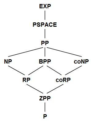
Here are the known relationships among the basic complexity classes that we've seen so far in this course. The relationships I didn't discuss explicitly are left as exercises for the reader (i.e., you).
It might surprise you that we still don't know whether BPP is contained in NP. But think about it: even if a BPP machine accepted with probability close to 1, how would you prove that to a deterministic polynomial-time verifier who didn't believe you? Sure, you could show the verifier some random runs of the machine, but then she'd always suspect you of skewing your samples to get a favorable outcome.
Fortunately, the situation isn't quite as pathetic as it seems: we at least know that BPP is contained in NPNP (that is, NP with NP oracle), and hence in the second level of the polynomial hierarchy PH. Sipser, Gács, and Lautemann proved that in 1983. I went through the proof in class, but I'm actually going to skip it in these notes, because it's a bit technical. If you want it, here it is.
Incidentally, while we know that BPP is contained in NPNP, we don't know anything similar for BQP, the class of problems solvable in polynomial time on a quantum computer. BQP hasn't yet made its official entrance in this course -- you'll have to wait a couple more lectures! -- but I'm trying to foreshadow it by telling you what it apparently isn't. In other words, what do we know to be true of BPP that we don't know to be true of BQP? Containment in PH is only the first of three examples we'll see in this lecture.
In complexity theory, it's hard to talk about randomness without also talking about a closely-related concept called nonuniformity. Nonuniformity basically means that you get to choose a different algorithm for each input length n. Now, why would you want such a stupid thing? Well, remember in Lecture 5 I showed you the Blum Speedup Theorem -- which says that it's possible to construct weird problems that admit no fastest algorithm, but only an infinite sequence of algorithms, with each one faster than the last on sufficiently large inputs? In such a case, nonuniformity would let you pick and choose from all algorithms, and thereby achieve the optimal performance. In other words, given an input of length n, you could simply pick the algorithm that's fastest for inputs of that particular length!
But even in a world with nonuniformity, complexity theorists believe there would still be strong limits on what could efficiently be computed. When we want to talk about those limits, we use a terminology invented by Karp and Lipton in 1982. Karp and Lipton defined the complexity class P/f(n), or P with f(n)-size advice, to consist of all problems solvable in deterministic polynomial time on a Turing machine, with help from an f(n)-bit "advice string" an that depends only on the input length n.
You can think of the polynomial-time Turing machine as a grad student, and the advice string an as wisdom from the student's advisor. Like most advisors, this one is infinitely wise, benevolent, and trustworthy. He wants nothing more than to help his students solve their respective thesis problems: that is, to decide whether their respective inputs x in {0,1}n are yes-inputs or no-inputs. But also like most advisors, he's too busy to find out what specific problems his students are working on. He therefore just doles out the same advice an to all of them, trusting them to apply it to their particular inputs x.
We'll be particularly interested in the class P/poly, which consists of all problems solvable in polynomial time using polynomial-size advice. In other words, P/poly is the union of P/nk over all positive integers k.
Now, is it possible that P = P/poly? As a first (trivial) observation, I claim the answer is no: P is strictly contained in P/poly, and indeed in P/1. In other words, even with a single bit of advice, you really can do more than with no advice. Why?
Right! Consider the following problem:
Given an input of length n, decide whether the nth Turing machine halts.
Not only is this problem not in P, it's not even computable -- for it's nothing other than a slow, "unary" encoding of the halting problem. On the other hand, it's easy to solve with a single advice bit an that depends only on the input length n. For that advice bit could just tell you what the answer is!
Here's another way to understand the power of advice: while the number of problems in P is only countably infinite, the number of problems in P/1 is uncountably infinite. (Why?)
On the other hand, just because you can solve vastly more problems with advice than you can without, that doesn't mean advice will help you solve any particular problem you might be interested in. Indeed, a second easy observation is that advice doesn't let you do everything: there exist problems not in P/poly. Why?
Well, here's a simple diagonalization argument. I'll actually show a stronger result, that there exist problems not in P/nlog n. Let M1,M2,M3,... be a list of polynomial-time Turing machines. Also, fix an input length n. Then I claim that there exists a Boolean function f:{0,1}n→{0,1} that the first n machines (M1,...,Mn) all fail to compute, even given any nlog n-bit advice string. Why? Just a counting argument: there are Boolean functions, but only n Turing machines and  advice strings. So choose such a function f for every n; you'll then cause each machine Mi to fail on all but finitely many input lengths. Indeed, we didn't even need the assumption that the Mi's run in polynomial time.
Of course, all this time we've been dancing around the real question: can advice help us solve problems that we actually care about, like the NP-complete problems? In particular, is NP contained in P/poly? Intuitively, it seems unlikely: there are exponentially many Boolean formulas of size n, so even if you somehow received a polynomial-size advice string from God, how would that help you to decide satisfiability for more than a tiny fraction of those formulas?
But -- and I'm sure this will come as a complete shock to you -- we can't prove it's impossible. Well, at least in this case we have a good excuse for our ignorance, since if P=NP, then obviously NP would be in P/poly as well. But here's a question: if we did succeed in proving P≠NP, then would we also have proved that NP is not in P/poly? In other words, would NP in P/poly imply P=NP? Alas, we don't even know the answer to that.
But as with BPP and NP, the situation isn't quite as pathetic as it seems. Karp and Lipton did manage to prove in 1982 that, if NP were contained in P/poly, then the polynomial hierarchy PH would collapse to the second level (that is, to NPNP). In other words, if you believe the polynomial hierarchy is infinite, then you must also believe that NP-complete problems are not efficiently solvable by a nonuniform algorithm.
This "Karp-Lipton Theorem" is the most famous example of a very large class of complexity results, a class that's been characterized as "if donkeys could whistle, then pigs could fly." In other words, if one thing no one really believes is true were true, then another thing no one really believes is true would be true! Intellectual onanism, you say? Nonsense! What makes it interesting is that the two things that no one really believes are true would've previously seemed completely unrelated to each other.
It's a bit of a digression, but the proof of the Karp-Lipton Theorem is more fun than a barrel full of carp. So let's see the proof right now. We assume NP is contained in P/poly; what we need to prove is that the polynomial hierarchy collapses to the second level -- or equivalently, that coNPNP = NPNP. So let's consider an arbitrary problem in coNPNP, like so:
For all n-bit strings x, does there exist an n-bit string y such that φ(x,y) evaluates to TRUE?
(Here φ is some arbitrary polynomial-size Boolean formula.)
We need to find an NPNP question -- that is, a question where the existential quantifier comes before the universal quantifier -- that has the same answer as the question above. But what could such a question possibly be? Here's the trick: we'll first use the existential quantifier to guess a polynomial-size advice string an. We'll then use the universal quantifier to guess the string x. Finally, we'll use the advice string an -- together with the assumption that NP is in P/poly -- to guess y on our own. Thus:
Does there exist an advice string an such that for all n-bit strings x, φ(x,M(x,an)) evaluates to TRUE?
Here M is a polynomial-time Turing machine that, given x as input and an as advice, outputs an n-bit string y such that φ(x,y) evaluates to TRUE whenever such a y exists. By one of your homework problems from last week, we can easily construct such an M provided we can solve NP-complete problems in P/poly.
Alright, I told you before that nonuniformity was closely related to randomness -- so much so that it's hard to talk about one without talking about the other. So in the rest of this lecture, I want to tell you about two connections between randomness and nonuniformity: a simple one that was discovered by Adleman in the 70's, and a deep one that was discovered by Impagliazzo, Nisan, and Wigderson in the 90's.
The simple connection is that BPP is contained in P/poly: in other words, nonuniformity is at least as powerful as randomness. Why do you think that is?
Well, let's see why it is. Given a BPP computation, the first thing we'll do is amplify the computation to exponentially small error. In other words, we'll repeat the computation (say) n2 times and then output the majority answer, so that the probability of making a mistake drops from 1/3 to roughly  . (If you're trying to prove something about BPP, amplifying to exponentially small error is almost always a good first step!)
Now, how many inputs are there of length n? Right: 2n. And for each input, only a fraction of random strings cause us to err. By the union bound (the most useful fact in all of theoretical computer science), this implies that at most a  fraction of random strings can ever cause us to err on inputs of length n. Since < 1, this means there exists a random string, call it r, that never causes us to err on inputs of length n. So fix such an r, feed it as advice to the P/poly machine, and we're done!
So that was the simple connection between randomness and nonuniformity. Before moving on to the deep connection, let me make two remarks.
- Even if P≠NP, you might wonder whether NP-complete problems can be solved in probabilistic polynomial time. In other words, is NP in BPP? Well, we can already say something concrete about that question. If NP is in BPP, then certainly NP is also in P/poly (since BPP is in P/poly). But that means PH collapses by the Karp-Lipton Theorem. So if you believe the polynomial hierarchy is infinite, then you also believe NP-complete problems are not efficiently solvable by randomized algorithms.
- If nonuniformity can simulate randomness, then can it also simulate quantumness? In other words, is BQP in P/poly? Well, we don't know, but it isn't considered likely. Certainly Adleman's proof that BPP is in P/poly completely breaks down if we replace the BPP by BQP. But this raises an interesting question: why does it break down? What's the crucial difference between quantum theory and classical probability theory, which causes the proof to work in the one case but not the other? I'll leave the answer as an exercise for you.
Alright, now for the deep connection. Do you remember the primality-testing problem from earlier in the lecture? Over the years, this problem crept steadily down the complexity hierarchy, like a monkey from branch to branch:
- It's obvious that primality-testing is in coNP.
- In 1975, Pratt showed it was in NP.
- In 1977, Solovay, Strassen, and Rabin showed it was in coRP.
- In 1992, Adleman and Huang showed it was in ZPP.
- In 2002, Agrawal, Kayal, and Saxena showed it was in P.
The general project of taking randomized algorithms and converting them to deterministic ones is called derandomization (a name only a theoretical computer scientist could love). The history of the primality-testing problem can only be seen as a spectacular success of this project. But with such success comes an obvious question: can every randomized algorithm be derandomized? In other words, does P equal BPP?
Once again the answer is that we don't know. Usually, if we don't know if two complexity classes are equal, the "default conjecture" is that they're different. And so it was with P and BPP -- (ominous music) -- until now. Over the last decade and a half, mounting evidence has convinced almost all of us that in fact P=BPP. In the remaining ten minutes of this lecture, we certainly won't be able to review this evidence in any depth. But let me quote one theorem, just to give you a flavor of it:
Theorem (Impagliazzo-Wigderson 1997): Suppose there exists a problem that's solvable in exponential time, and that's not solvable in subexponential time even with the help of a subexponential-size advice string. Then P=BPP.
Notice how this theorem relates derandomization to nonuniformity -- and in particular, to proving that certain problems are hard for nonuniform algorithms. The premise certainly seems plausible. From our current perspective, the conclusion (P=BPP) also seems plausible. And yet the two seem to have nothing to do with each other. So, this theorem might be characterized as "If donkeys can bray, then pigs can oink."
Where does this connection between randomness and nonuniformity come from? It comes from the theory of pseudorandom generators. We're gonna see a lot more about pseudorandom generators in the next lecture, when we talk about cryptography. But basically, a pseudorandom generator is just a function that takes as input a short string (called the seed), and produces as output a long string, in such a way that, if the seed is random, then the output looks random. Obviously the output can't be random, since it doesn't have enough entropy: if the seed is k bits long, then there are only 2k possible output strings, regardless of how long those output strings are. What we ask, instead, is that no polynomial-time algorithm can successfully distinguish the output of the pseudorandom generator from "true" randomness. Of course, we'd also like for the function mapping the seed to the output to be computable in polynomial time.
Already in 1982, Andy Yao realized that, if you could create a "good enough" pseudorandom generator, then you could prove P=BPP. Why? Well, suppose that for any integer k, you had a way of stretching an O(log n)-bit seed to an n-bit output in polynomial time, in such a way that no algorithm running in nk time could successfully distinguish the output from true randomness. And suppose you had a BPP machine that ran in nk time. In that case, you could simply loop over all possible seeds (of which there are only polynomially many), feed the corresponding outputs to the BPP machine, and then output the majority answer. The probability that the BPP machine accepts given a pseudorandom string has to be about the same as the probability that it accepts given a truly random string -- since otherwise the machine would be distinguishing random strings from pseudorandom ones, contrary to assumption!
But what's the role of nonuniformity in all this? Well, here's the point: in addition to a random (or pseudorandom) string, a BPP machine also receives an input, x. And we need the derandomization to work for every x. But that means that, for the purposes of derandomization, we must think of x as an advice string provided by some superintelligent adversary for the sole purpose of foiling the pseudorandom generator. You see, this is why we had to assume a problem that was hard even in the presence of advice: because we need to construct a pseudorandom generator that's indistinguishable from random even in the presence of the "adversary," x.
(That reminds me of something: why are there so many Israelis in complexity, and particularly in the more cryptographic kinds of complexity? I have a theory about this: it's because complexity is basically mathematicized paranoia. It's that field where, whenever anyone else has any choice in what to do, you immediately assume that person will do the worst possible thing to you and proceed accordingly.)
To summarize: if we could prove that certain problems are sufficiently hard for nonuniform algorithms, then we would prove P=BPP.
This leads to my third difference between BPP and BQP: while most of us believe that P=BPP, most of us certainly don't believe that P=BQP. (Indeed we can't believe that, if we believe factoring is hard for classical computers.) We don't have any "dequantization" program that's been remotely as successful as the derandomization program. Once again, it would seem there's a crucial difference between quantum theory and classical probability theory, which allows certain ideas (like those of Sipser-Gács-Lautemann, Adleman, and Impagliazzo-Wigderson) to work for the latter but not for the former.
Incidentally, over the last few years, Kabanets, Impagliazzo, and others managed to obtain a sort of converse to the derandomization theorems. What they've shown is that, if we want to prove P=BPP, then we'll have to prove that certain problems are hard for nonuniform algorithms. This could be taken as providing some sort of explanation for why, assuming P=BPP, no one has yet managed to prove it. Namely, it's because if you want to prove P=BPP, then you'll have to prove certain problems are hard -- and if you could prove those problems were hard, then you would be (at least indirectly) attacking questions like P versus NP. In complexity theory, pretty much everything eventually comes back to P versus NP.
Puzzles for Thursday
- You and a friend want to flip a coin, but the only coin you have is crooked: it lands heads with some fixed but unknown probability p. Can you use this coin to simulate a fair coin flip? (I mean perfectly fair, not just approximately fair.)
- n people are standing in a circle. They're each wearing either a red hat or a blue hat, assigned uniformly and independently at random. They can each see everyone else's hats but not their own. They want to vote on whether the number of red hats is even or odd. Each person votes at the same time, so that no one's vote depends on anyone else's. What's the maximum probability with which the people can win this game? (By "win," I mean that their vote corresponds to the truth.) Assume for simplicity that n is odd.
[Discussion of this lecture on blog]
[← Previous lecture | Next lecture →]
[Return to PHYS771 home page]